| Multivariate Pattern Analysis in Python |
| Multivariate Pattern Analysis in Python |
PyMVPA includes a number of ready-to-use classifiers, which are described in the following sections. All classifiers implement the same, very simple interface. Each classifier object takes all relevant parameters as arguments to its constructor. Once instantiated, the classifier object’s train() method can be called with some dataset. This trains the classifier using all samples in the respective dataset.
The major task for a classifier is to make predictions. Predictions are made by calling the classifier’s predict() method with one or multiple data samples. predict() operates on pure sample data and not datasets, as in some cases the true label for a sample might be totally unknown.
This examples demonstrates the typical daily life of a classifier.
>>> import numpy as N
>>> from mvpa.clfs.knn import kNN
>>> from mvpa.datasets import Dataset
>>> training = Dataset(samples=N.array(
...                                N.arange(100),ndmin=2, dtype='float').T,
...                    labels=[0] * 50 + [1] * 50)
>>> rand100 = N.random.rand(10)*100
>>> validation = Dataset(samples=N.array(rand100, ndmin=2, dtype='float').T,
...                      labels=[ int(i>50) for i in rand100 ])
>>> clf = kNN(k=10)
>>> clf.train(training)
>>> N.mean(clf.predict(training.samples) == training.labels)
1.0
>>> N.mean(clf.predict(validation.samples) == validation.labels)
1.0
Two datasets with 100 and 10 samples each are generated. Both datasets only have one feature and the associated label is 0 if the feature value is below 50 or 1 otherwise. The larger dataset contains all integers in the interval (0,100) and is used to train the classifier. The smaller is used as a validation dataset, to check whether the classifier learned something that generalizes well across samples not included in the training dataset. In this case the validation dataset consists of 10 random floating point values in the interval (0,100).
The classifier in this example is a kNN (k-Nearest-Neighbour) classifier that makes use of the 10 nearest neighbours of a data sample to make its predictions (k=10). One can see that after the training the classifier performs optimally on the training dataset as well as on the validation data samples.
The choice of the classifier in the above example is more or less arbitrary. Any classifier in PyMVPA could be used in place of kNN. This demonstrates another useful feature of PyMVPA’s classifiers. Due to the high-level abstraction and the simple interface, almost all classifiers can be combined with most algorithms in PyMVPA. This makes it very easy to test different classifiers on some dataset (see Fig. 1).
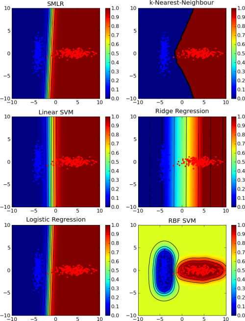
A comparison of the behavior of different classifiers (k-Nearest-Neighbour, linear SVM, logistic regression, ridge regression and SVM with radial basis function kernel) on a simple classification problem. The code to generate these figure can be found in the pylab_2d.py example in the Simple Plotting of Classifier Behavior section.
Before looking at the different classifiers in more detail, it is important to mention another feature common to all of them. While their interface is simple, classifiers are in no way limited to report only predictions. All classifiers implement an additional interface: Objects of any class that are derived from ClassWithCollections have attributes (we refer to such attributes as state variables), which are conditionally computed and stored by PyMVPA. Such conditional storage and access is handy if a variable of interest might consume a lot of memory or needs intensive computation, and not needed in most (or in some) of the use cases.
For instance, the Classifier class defines the trained_labels state variable, which just stores the unique labels for which the classifier was trained. Since trained_labels stores meaningful information only for a trained classifier, attempt to access ‘clf.trained_labels’ before training would result in an error,
>>> from mvpa.misc.exceptions import UnknownStateError
>>> try:
...     untrained_clf = kNN()
...     labels = untrained_clf.trained_labels
... except UnknownStateError:
...     "Does not work"
'Does not work'
since the classifier has not seen the data yet and, thus, does not know the labels. In other words, it is not yet in the state to know anything about the labels. Any state variable can be enabled or disabled on per instance basis at any time of the execution (see ClassWithCollections).
To continue the last example, each classifier, or more precisely every stateful object, can be asked to report existing state-related attributes:
>>> list_with_verbose_explanations = clf.states.listing
‘clf.states’ is an instance of StateCollection class which is a container for all state variables of the given class. Although values can be queried or set (if state is enabled) operating directly on the stateful object
>>> clf.trained_labels
array([0, 1])
any other operation on the state (e.g. enabling, disabling) has to be carried out through the states attribute.
>>> print clf.states
states{trained_dataset predicting_time*+ training_confusion predictions*+...}
>>> clf.states.enable('values')
>>> print clf.states
states{trained_dataset predicting_time*+ training_confusion predictions*+...}
>>> clf.states.disable('values')
A string representation of the state collection mentioned above lists all state variables present accompanied with 2 markers: ‘+’ for an enabled state variable, and ‘*’ for a variable that stores some value (but might have been disabled already and, therefore, would have no ‘+’ and attempts to reassign it would result in no action).
By default all classifiers provide state variables values, predictions. The latter is simply the set of predictions that was returned by the last call to the objects predict() method. The former is heavily classifier-specific. By convention the values key provides access to the raw values that a classifier prediction is based on. Depending on the classifier, this information might required significant resources when stored. Therefore all states can be disabled or enabled (states.disable(), states.enable()) and their current status can be queried like this:
>>> clf.states.isActive('predictions')
True
>>> clf.states.isActive('values')
False
States can be enabled or disabled during stateful object construction, if enable_states or disable_states (or both) arguments, which store the list of desired state variables names, passed to the object constructor. Keyword ‘all’ can be used to select all known states for that stateful object.
The TransferError class provides a convenient way to determine the transfer error of a trained classifier on some validation dataset, i.e. the accuracy of the classifier’s predictions on a novel, independent dataset. A TransferError object is instanciated by passing a classifier object to the constructor. Optionally a custom error function can be specified (see errorfx argument).
To compute the transfer error simply call the object with a validation dataset. The computed error value is returned. TransferError also supports a state variable confusion that contains the full confusion matrix of the predictions made on the validation dataset. The confusion matrix is disabled by default.
If the TransferError object is called with an optional training dataset, the contained classifier is first training using this dataset before predictions on the validation dataset are made.
>>> from mvpa.clfs.transerror import TransferError
>>> clf = kNN(k=10)
>>> terr = TransferError(clf)
>>> terr(validation, training )
0.0
Often one is not only interested in a single transfer error on one validation or test dataset, but on a cross-validated estimate of the transfer error. A popular method is the so-called leave-one-out cross-validation.
The CrossValidatedTransferError class provides a simple way to compute such measure. It utilizes a TransferError object and a Splitter. When called with a Dataset the splitter generates splits of the Dataset and the transfer error for all splits is computed by training on one of the splitted datasets and making predictions on the other. By default the mean of transfer errors is returned (but the actual combiner function is customizable).
The following example shows the minimal code for a leave-one-out cross-validation reusing the transfer error object from the previous example and some Dataset data.
>>> # create some dataset
>>> from mvpa.misc.data_generators import normalFeatureDataset
>>> data = normalFeatureDataset(perlabel=50, nlabels=2,
...                             nfeatures=20, nonbogus_features=[3, 7],
...                             snr=3.0)
>>> # now cross-validation
>>> from mvpa.algorithms.cvtranserror import CrossValidatedTransferError
>>> from mvpa.datasets.splitters import NFoldSplitter
>>> cvterr = CrossValidatedTransferError(terr,
...                                      NFoldSplitter(cvtype=1),
...                                      enable_states=['confusion'])
>>> error = cvterr(data)
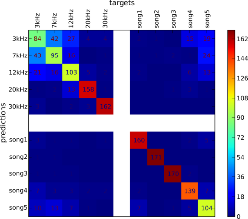
PyMVPA is equipped with easy ways to have a glance overview over the generalization performance of a cross-validated classifier. Such summary is provided by instances of a ConfusionMatrix class, and is accompanied by various performance metrics. For example, the 8-fold cross-validation of the dataset with 8 labels with the SMLR classifier produced the following confusion matrix:
>>> # Simple 'print cvterr.confusion' provides the same output
>>> # without the description of abbreviations
>>> print cvterr.confusion.asstring(description=True) \
...
--------.        3kHz  7kHz  12kHz 20kHz 30kHz song1 song2 song3 song4 song5
predict.\targets 38    39    40    41    42    43    44    45    46    47
         `------ ---- ----- ----- ----- ----- ----- ----- ----- ----- -----  P'  N'  FP  FN   PPV  NPV  TPR  SPC  FDR  MCC
       3kHz / 38 84    42    27     4     4     2     1     0    15    19   198 1351 114 90  0.42 0.93 0.48 0.92 0.58 0.36
       7kHz / 39 43    94    16     0     1     1     1     2     1    24   183 1331 89  80  0.51 0.94 0.54 0.93 0.49 0.43
      12kHz / 40 21    16    103    5     2     2     0     0     6    13   168 1312 65  70  0.61 0.95  0.6 0.95 0.39 0.51
      20kHz / 41  1     2    13    158    1     0     0     1     3     1   180 1202 22  15  0.88 0.99 0.91 0.98 0.12 0.77
      30kHz / 42  3     0     2     3    162    0     0     0     0     0   170 1194  8  11  0.95 0.99 0.94 0.99 0.05 0.82
      song1 / 43  3     1     1     0     1    160    0     0     2     5   173 1199 13  14  0.92 0.99 0.92 0.99 0.08  0.8
      song2 / 44  1     1     0     0     0     0    171    0     0     0   173 1176  2   2  0.99   1  0.99   1  0.01 0.86
      song3 / 45  1     1     1     0     0     0     0    170    2     0   175 1179  5   4  0.97   1  0.98   1  0.03 0.84
      song4 / 46  7     3     3     2     2     2     0     0    139    7   165 1240 26  34  0.84 0.97  0.8 0.98 0.16 0.71
      song5 / 47 10    14     7     1     0     7     0     1     5    104  149 1310 45  69   0.7 0.95  0.6 0.97  0.3 0.55
Per target:      ---- ----- ----- ----- ----- ----- ----- ----- ----- -----
      P          174   174   173   173   173   174   173   174   173   173
      N         1560  1560  1561  1561  1561  1560  1561  1560  1561  1561
      TP         84    94    103   158   162   160   171   170   139   104
      TN        1261  1251  1242  1187  1183  1185  1174  1175  1206  1241
Summary\Means:  ---- ----- ----- ----- ----- ----- ----- ----- ----- ----- 173 1249 38  39  0.78 0.97 0.78 0.97 0.22 0.66
     ACC        0.78
     ACC%       77.57
  # of sets       8

Statistics computed in 1-vs-rest fashion per each target.
Abbreviations (for details see http://en.wikipedia.org/wiki/ROC_curve):
 TP : true positive (AKA hit)
 TN : true negative (AKA correct rejection)
 FP : false positive (AKA false alarm, Type I error)
 FN : false negative (AKA miss, Type II error)
 TPR: true positive rate (AKA hit rate, recall, sensitivity)
      TPR = TP / P = TP / (TP + FN)
 FPR: false positive rate (AKA false alarm rate, fall-out)
      FPR = FP / N = FP / (FP + TN)
 ACC: accuracy
      ACC = (TP + TN) / (P + N)
 SPC: specificity
      SPC = TN / (FP + TN) = 1 - FPR
 PPV: positive predictive value (AKA precision)
      PPV = TP / (TP + FP)
 NPV: negative predictive value
      NPV = TN / (TN + FN)
 FDR: false discovery rate
      FDR = FP / (FP + TP)
 MCC: Matthews Correlation Coefficient
      MCC = (TP*TN - FP*FN)/sqrt(P N P' N')
 # of sets: number of target/prediction sets which were provided
In addition to the abusively informative textual representation, there is an alternative graphical representation of the confusion matrix via the plot() method of a ConfusionMatrix:
>>> import pylab as P
>>> cvterr.confusion.plot() \
...
>>> P.show() \
...
PyMVPA provides a number of learning methods (i.e. classifiers or regression algorithms) that can be plug into the various algorithms that are also part of the framework. Most importantly they all can be combined or enhanced with Meta-Classifiers.
The kNN classifier makes predictions based on the labels of nearby samples. It currently uses Euclidean distance to determine the nearest neighbours, but future enhancements may include support for other kernels.
The penalized logistic regression (PLR) is similar to the ridge in that it has a penalty term, however, it is trained to predict a binary outcome by means of the logistic function (Wikipedia entry about logistic regression).
Ridge regression (aka Tikhonov regularization) is a variant of a linear regression (Wikipedia entry about ridge regression).
The ridge regression classifier (RidgeReg) performs a simple linear regression with a penalty parameter to help avoid over-fitting. The regression inserts an intercept term so that you do not have to center your data.
Sparse Multinomial Logistic Regression (SMLR; Krishnapuram et al., 2005) is a fast multi-class classifier that can easily deal with high-dimensional problems (research paper about SMLR). PyMVPA includes two implementations: one in pure Python and a faster one that makes use of a C extension for the performance critical pieces of the code.
Support vector machine (Vapnik, 1995) classifiers (and regressions) are popular since they can deal with very high dimensional problems (Wikipedia entry about SVM), while maintaining reasonable generalization performance.
The support vector machine classes provide a family of classifiers by wrapping LIBSVM and Shogun libraries, with corresponding base classes SVM and SVM accordingly. By default SVM class is bound to LIBSVM’s implementation if such is available (shogun otherwise).
While any SVM class provides a complete interface, the others child classes make it easy to run some subset of standard classifiers, such as linear SVM, with a default set of parameters (see LinearCSVMC, LinearNuSVMC, RbfNuSVMC and RbfCSVMC).
This section has been contributed by James M. Hughes.
A meta-classifier is essentially a blanket term used to describe all classes that appear functionally equivalent to a regular Classifier, but which in reality provide some extra amount of functionality on top of a normal classifier. Furthermore, they generally do not implement a Classifier per se, but rather take a Classifier as input. The methods then typically called on a classifier (e.g., train or predict) can be called on the meta-classifier, but will call the input classifier’s routines, before or after some other function that the meta-classifier provides.
At present, there are two primary meta-classifiers implemented in the PyMVPA package, beneath which there are several specific options:
Within these more general categories, specific classifiers are implemented. For example, there are several BoostedClassifier subclasses:
Furthermore, there are also several ProxyClassifier subclasses:
Classifiers such as the FeatureSelectionClassifier are particularly useful because they simplify the process of selecting features and then using only that subset of features to classify novel exemplars (the predict stage). They become even more powerful when combined with SplitClassifier, so that even the task of withholding certain data points to create statistically valid training and testing datasets is abstracted and wrapped up within a single object (and, ultimately, very few method calls). Consider the following code, which can be found in mvpa/clfs/warehouse.py:
>>> from mvpa.clfs.meta import SplitClassifier, FeatureSelectionClassifier
>>> from mvpa.clfs.svm import LinearCSVMC
>>> from mvpa.clfs.transerror import ConfusionBasedError
>>> from mvpa.featsel.rfe import RFE
>>> from mvpa.featsel.helpers import FractionTailSelector
>>>
>>> rfesvm_split = SplitClassifier(LinearCSVMC())
>>> clf = \
...  FeatureSelectionClassifier(
...   clf = LinearCSVMC(),
...   # on features selected via RFE
...   feature_selection = RFE(
...       # based on sensitivity of a clf which does
...       # splitting internally
...       sensitivity_analyzer=rfesvm_split.getSensitivityAnalyzer(),
...       transfer_error=ConfusionBasedError(
...          rfesvm_split,
...          confusion_state="confusion"),
...          # and whose internal error we use
...       feature_selector=FractionTailSelector(
...                          0.2, mode='discard', tail='lower'),
...                          # remove 20% of features at each step
...       update_sensitivity=True),
...       # update sensitivity at each step
...   descr='LinSVM+RFE(splits_avg)' )
This analysis combines the FeatureSelectionClassifier and the SplitClassifier to perform internal splitting of the data and then perform FeatureSelection based on those splits. Such analyses can be easily created due to the straightforward way that classifier and meta-classifiers can be combined. Please refer to the relevant documentation sections for more information about the specifics of each meta-classifier.
Some classifiers have ability to provide quick (i.e in terms of performance) re-training if they were previously trained, and only part of their specification got changed. For instance, for kernel-based classifier (e.g. GPR) it makes no sense to recompute kernel matrix, if only a classifier (not kernel) parameter (e.g. sigma_noise) was changed. Another similar usecase: for null-hypothesis statistical testing it might be needed to train classifier multiple times on a randomized set of labels.
Only classifiers which have retrainable in their _clf_internals are capable of efficient retraining. To enable retraining, just provide retrainable=True to the constructor of the classifier. Internally retrainable classifiers will try to deduce what was changed in the specification of the classifier (e.g. training/testing datasets, parameters) and act accordingly. To reduce training/prediction time even more, classifier might directly be instructed with what aspects were changed. It must be previously trained / predicted, so later on retrain() and repredict() methods could be called. repredict() can be called only with the same data, for which it was earlier predicted. See API doc for more information.
Implementation of efficient retraining is not straightforward, thus it is strongly advised to
- enable CHECK_RETRAIN debug target while developing the code for analysis. That might guard you against obvious misuses of retraining feature, as well as to spot bugs in the code
- validate on a simple dataset that analysis code provides the same results if classifier was created retrainable or not
To facilitate easy trial of different classifiers for any specific task, Warehouse of classifiers clfs.warehouse.clfs was defined to create a sample collection of some commonly used parameterizations of the classifiers present in PyMVPA. Such collection can be queried by any set of known keywords/tags with tags prefixed with ! being excluded:
>>> from mvpa.clfs.warehouse import clfswh
>>> tryme = clfswh['multiclass', '!svm']
to simply sweep through classifiers which are capable of multiclass classification and are not SVM based.