This content refers to the previous stable release of PyMVPA. Please visit www.pymvpa.org for the most recent version of PyMVPA and its documentation.

Generating Topography plots

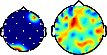
Example demonstrating a topography plot.

from mvpa.suite import *

# Sanity check if we have griddata available
externals.exists("griddata", raiseException=True)

# EEG example splot
P.subplot(1, 2, 1)

# load the sensor information from their definition file.
# This file has sensor names, as well as their 3D coordinates
sensors=XAVRSensorLocations(os.path.join(pymvpa_dataroot, 'xavr1010.dat'))

# make up some artifical topography
# 'enable' to channels, all others set to off ;-)
topo = N.zeros(len(sensors.names))
topo[sensors.names.index('O1')] = 1
topo[sensors.names.index('F4')] = 1

# plot with sensor locations shown
plotHeadTopography(topo, sensors.locations(), plotsensors=True)


# MEG example plot
P.subplot(1, 2, 2)

# load MEG sensor locations
sensors=TuebingenMEGSensorLocations(
            os.path.join(pymvpa_dataroot, 'tueb_meg_coord.xyz'))

# random values this time
topo = N.random.randn(len(sensors.names))

# plot without additional interpolation
plotHeadTopography(topo, sensors.locations(),
                   interpolation='nearest')


if cfg.getboolean('examples', 'interactive', True):
    # show all the cool figures
    P.show()

The ouput of the provided example should look like

See also

The full source code of this example is included in the PyMVPA source distribution (doc/examples/topo_plot.py).