This content refers to the previous stable release of PyMVPA. Please visit www.pymvpa.org for the most recent version of PyMVPA and its documentation.

Self-organizing Maps

This is a demonstration of how a self-organizing map (SOM), also known as a Kohonen network, can be used to map high-dimensional data into a two-dimensional representation. For the sake of an easy visualization ‘high-dimensional’ in this case is 3D.

In general, SOMs might be useful for visualizing high-dimensional data in terms of its similarity structure. Especially large SOMs (i.e. with large number of Kohonen units) are known to perform mappings that preserve the topology of the original data, i.e. neighboring data points in input space will also be represented in adjacent locations on the SOM.

The following code shows the ‘classic’ color mapping example, i.e. the SOM will map a number of colors into a rectangular area.

from mvpa.suite import *

First, we define some colors as RGB values from the interval (0,1), i.e. with white being (1, 1, 1) and black being (0, 0, 0). Please note, that a substantial proportion of the defined colors represent variations of ‘blue’, which are supposed to be represented in more detail in the SOM.

colors = [[0., 0., 0.],
          [0., 0., 1.],
          [0., 0., 0.5],
          [0.125, 0.529, 1.0],
          [0.33, 0.4, 0.67],
          [0.6, 0.5, 1.0],
          [0., 1., 0.],
          [1., 0., 0.],
          [0., 1., 1.],
          [1., 0., 1.],
          [1., 1., 0.],
          [1., 1., 1.],
          [.33, .33, .33],
          [.5, .5, .5],
          [.66, .66, .66]]

# store the names of the colors for visualization later on
color_names = \
        ['black', 'blue', 'darkblue', 'skyblue',
         'greyblue', 'lilac', 'green', 'red',
         'cyan', 'violet', 'yellow', 'white',
         'darkgrey', 'mediumgrey', 'lightgrey']

Since we are going to use a mapper, we will put the color vectors into a dataset. To be able to do this, we will assign an arbitrary label, although it will not be used at all, since this SOM mapper uses an unsupervised training algorithm.

ds = Dataset(samples=colors, labels=1)

Now we can instantiate the mapper. It will internally use a so-called Kohonen layer to map the data onto. We tell the mapper to use a rectangular layer with 20 x 30 units. This will be the output space of the mapper. Additionally, we tell it to train the network using 400 iterations and to use custom learning rate.

som = SimpleSOMMapper((20, 30), 400, learning_rate=0.05)

Finally, we train the mapper with the previously defined ‘color’ dataset.

som.train(ds)

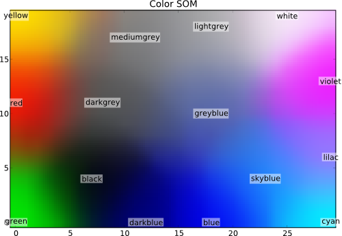
Each unit in the Kohonen layer can be treated as a pointer into the high-dimensional input space, that can be queried to inspect which input subspaces the SOM maps onto certain sections of its 2D output space. The color-mapping generated by this example’s SOM can be shown with a single matplotlib call:

P.imshow(som.K, origin='lower')

And now, let’s take a look onto which coordinates the initial training prototypes were mapped to. The get those coordinates we can simply feed the training data to the mapper and plot the output.

mapped = som(colors)

P.title('Color SOM')
# SOM's kshape is (rows x columns), while matplotlib wants (X x Y)
for i, m in enumerate(mapped):
    P.text(m[1], m[0], color_names[i], ha='center', va='center',
           bbox=dict(facecolor='white', alpha=0.5, lw=0))

The text labels of the original training colors will appear at the ‘mapped’ locations in the SOM – and should match with the underlying color.

# show the figure
if cfg.getboolean('examples', 'interactive', True):
    P.show()

The following figure shows an exemplary solution of the SOM mapping of the 3D color-space onto the 2D SOM node layer:

See also

The full source code of this example is included in the PyMVPA source distribution (doc/examples/som.py).