This content refers to the previous stable release of PyMVPA. Please visit www.pymvpa.org for the most recent version of PyMVPA and its documentation.

Curve-Fitting

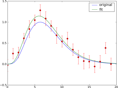
An example showing how to fit an HRF model to noisy peristimulus time-series data.

First, importing the necessary pieces:

import numpy as N
import pylab as P

from mvpa.misc.plot import plotErrLine
from mvpa.misc.fx import singleGammaHRF, leastSqFit
from mvpa import cfg

Now, we generate some noisy “trial time courses” from a simple gamma function (40 samples, 6s time-to-peak, 7s FWHM and no additional scaling:

a = N.asarray([singleGammaHRF(N.arange(20), A=6, W=7, K=1)] * 40)
# get closer to reality with noise
a += N.random.normal(size=a.shape)

Fitting a gamma function to this data is easy (using resonable seeds for the parameter search (5s time-to-peak, 5s FWHM, and no scaling):

fpar, succ = leastSqFit(singleGammaHRF, [5,5,1], a)

Generate high-resultion curves for the ‘true’ time course and the fitted one for visualization and plot them together with the data:

x = N.linspace(0,20)
curves = [(x, singleGammaHRF(x, 6, 7, 1)),
          (x, singleGammaHRF(x, *fpar))]

# plot data (with error bars) and both curves
plotErrLine(a, curves=curves, linestyle='-')

# add legend to plot
P.legend(('original', 'fit'))

if cfg.getboolean('examples', 'interactive', True):
    # show the cool figure
    P.show()

The ouput of the provided example should look like

See also

The full source code of this example is included in the PyMVPA source distribution (doc/examples/curvefitting.py).